Atom-loss validation and benchmarks
Inspect independent controls, measured workflows, and the data behind every figure. Start with the findings; open the methods when you need them.
The decoder methods follow the pinned Pauli Envelope paper, v2. Results here validate the recorded implementation and workload; they do not claim reproduction of every result in the paper. Run the tutorial for the physical loss model, gadget and public/private data boundary.
What the evidence supports
Independent checksSampling, decoding and a finite real-circuit chain have separate controls.
Conditioning helps in the tested settingIn the 15,000-shot tradeoff experiment: 35 failures with envelope weights, 61 with fixed weights.
No universal backend rankingWith identical envelope weights, RustQEC and PyMatching have the same total failure count at every tested setting across three new seeds.
These experiments exercise loss-visible Mid-SWAP circuits and the public-input decoding tutorial. They measure a defined workload; they do not establish a loss threshold or support for arbitrary circuits.
Independent correctness checks
A separate Python reference samples persistent loss histories and lowers them to ordinary Stim circuits. It removes gates touching absent atoms, preserves surviving-wire statistics, and restores a wire only on reset. It does not call RustQEC's sampler or loss compiler.
Sampling: coverage & negative controls
12 small circuits, 32,768 shots per implementation per circuit, checked against complete joint output distributions. Four deterministic cases also have hand-computed answers. Sixteen analytic channel checks cover live, lost and reset-restored wires. Another 26 distribution probes resolve every Pauli component through Bell-pair readout and check X/Y/Z product-basis joint distributions, both bit marginals and both loss directions. Deleting any of the five Pauli noise channels from native input must fail, including complete deletion of two-qubit depolarization. Replacing depolarization with noise on only one wire, independent X errors, or a single Pauli direction must also fail. A deliberately incorrect skipped-gate rule is detected.
Actual low noise and data export: coverage & negative controls
fifteen analytic probes use at least 262,144 shots each at Pauli probability 0.001 and the five benchmark loss rates plus their two-qubit half rates, with exact binomial count intervals. An independent 65,536-shot check exercises the real Mid-SWAP blinded data exporter, comparing measurement bits, detectors and selected joints within each logical input. It also checks detector rates when no loss is visible and independently verifies every scoring answer from observable parity and the private input mask. Deleting low-rate Pauli noise, loss, or both must fail separately. These correctness samples do not increase the 5,000-shot accuracy benchmark’s sample size.
Decoding: coverage & negative controls
hand-derived three- and five-wire parity graphs, all 1,088 flag/value rows, and exhaustive correction enumeration. Both matching backends must return a minimum-weight logical answer; exact ties are allowed. Lost-value placeholders and the loss-to-edge mapping are checked explicitly. A five-wire case has different unique optimal answers with and without conditioning: an actual decoder that ignores conditioning must fail, as must an intentionally flipped prediction.
Real circuit chain: coverage & negative controls
a two-round, distance-3 Mid-SWAP fixture with 16 detectors. Independently generated single-fault records exercise four loss histories. Stim-derived fault distributions, 897 Pauli probes and canonical syndromes check the native compiler; exact parity-state enumeration scores all 752 deterministic reference-witness rows through native matching/MLE and the actual PyMatching and native offline batch adapters. Both batch adapters must reject empty exported graphs, missing loss mappings and corrupted relative weights. Row-level oracle answers and predictions are retained; CI reruns and compares the report. This covers the finite fixture and four loss histories.
The real-circuit check covers a finite fixture and the declared envelope model. MLE is checked against its fault-configuration objective after independently validating the native model distribution; this does not establish physical logical-class Bayes optimality or prove arbitrary compiler inputs correct.
Sampling check report · Exhaustive matching check report · Mid-SWAP chain check report · Exact test circuit
Sampling workflow costs
| Distance (rounds = d) | RustQEC | Python + Stim correctness reference |
|---|---|---|
| d = 3 | 8.35(7.66–9.22) | 16.06(15.41–16.94) |
| d = 5 | 54.68(54.5–54.76) | 182.67(176.51–182.86) |
| d = 7 | 257.19(256.71–257.84) | 603.2(602.25–605.15) |
Pauli probability 0.001; configured pLoss = 0.003 (two-qubit targets: pLoss/2). Both produce loss-visible records and pack b8. Rust uses two warmups; the reference uses one. Imports, process startup and file I/O are excluded. All sampling measurements.
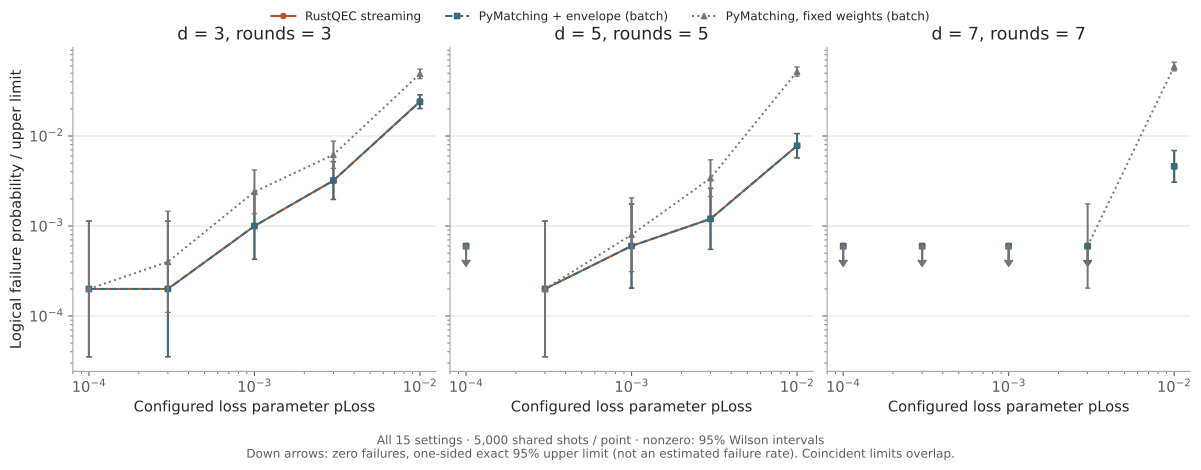
Failures across the loss sweep
Detail: nonzero failure rates at d = 3 and d = 5
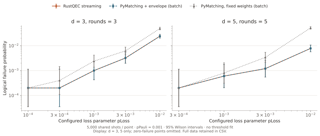
The PyMatching envelope adapter uses the same compiled graph, canonical syndromes and loss-conditioned weights as RustQEC. Fixed-weight PyMatching is an ablation: it removes loss-conditioned edge weights while retaining the same canonical syndromes. It therefore tests the value of this weighting rule, rather than removing every use of loss information.
Many low-loss points have only 0–5 failures in 5,000 shots and cannot resolve small differences. Overlapping intervals do not establish an accuracy ranking. Distances use different experiment durations, and these points are insufficient for a threshold estimate.
Accuracy and workflow time
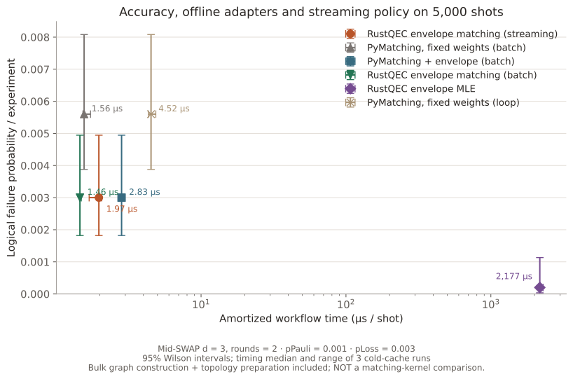
Comparison setup & timing boundaries
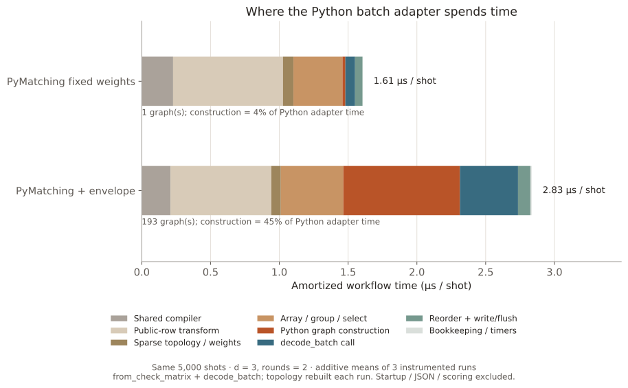
Fixed-weight PyMatching is a weight-conditioning ablation: it retains the shared canonical syndromes and graph, and is not a decoder deprived of all loss information. The main PyMatching paths use official from_check_matrix bulk graph construction and decode_batch; the fixed-weight per-shot loop is retained as a control with identical predictions. Conditioned batches group shots by visible loss pattern and restore their original order. This offline policy differs from RustQEC's streaming cache.
Backend order rotates between timing repetitions. Every repetition freshly measures compilation, public-row transformation and sparse topology/weight preparation. Python timings include array conversion, grouping, graph construction, decoding, reordering and output write/flush; JSON transport/loading, startup and scoring are excluded. Native decode includes buffered reads and output packing/flush; exporter transformation includes input reads. The added native offline adapter uses the same exported public graph and offline grouping policy as PyMatching; both include b8 output write/flush and exclude JSON transport. The streaming CLI remains a separate policy. These are adapter costs, not isolated kernel benchmarks or online tail latency.
These three timing repetitions reuse one 5,000-shot corpus; they are not 15,000 independent accuracy samples. On this setting, conditioning versus fixed weights has 0 conditioned-only failures and 13 fixed-only failures. That paired observation supports improvement here, not across every setting. MLE's 1 failure in 5,000 shots has substantial relative uncertainty and concerns its declared fault-configuration objective.
Accuracy across three seeds
Three seeds were fixed before sampling, with 5,000 shots each at every setting. This separate experiment adds 15,000 independent shots per setting; timing repeats do not increase its sample size. Each seed's results remain available.
With identical envelope weights, RustQEC and PyMatching have the same total failure count at every setting across these three seeds. In the 15,000-shot tradeoff setting, each has 35 failures, compared with 61 for fixed-weight PyMatching. The paired evidence supports the benefit of loss-conditioned weights at this setting; it does not establish an accuracy advantage of the Rust backend.
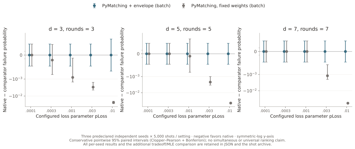
All per-seed counts and paired intervals · 48 corpora and 147 predictions, with standalone rescorer (ZIP) · Seed experiment provenance
Offline and streaming workflows
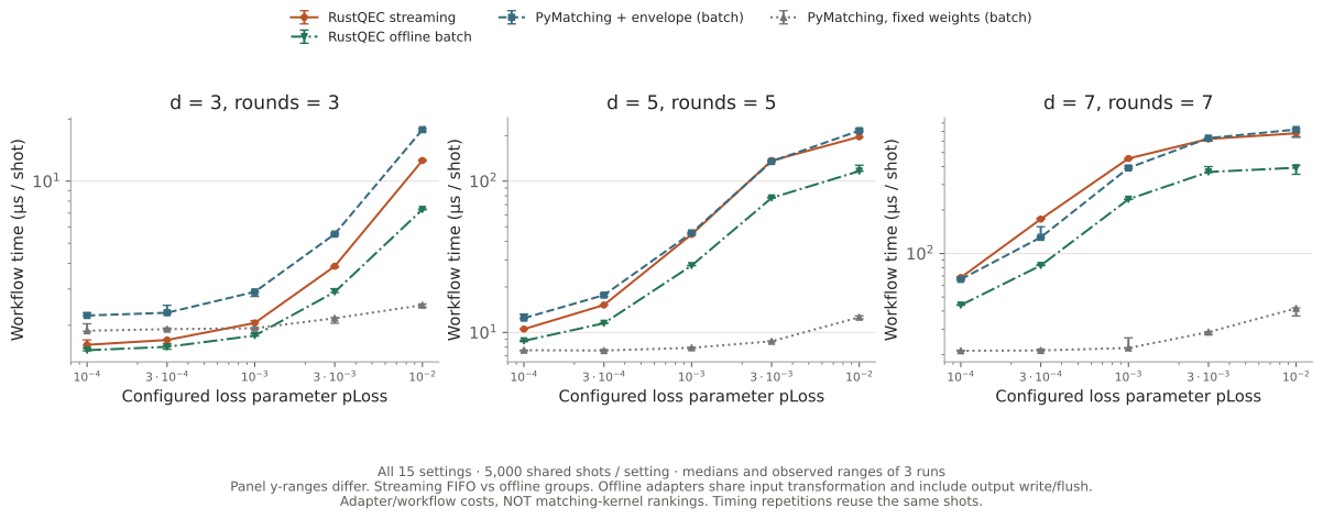
Native offline and Python both group the entire batch by visible loss pattern and build one graph per pattern; both include output write/flush. Native streaming uses a bounded FIFO cache and is shown as a separate policy. This figure compares these workflows, not matching kernels. Download all timing repetitions, graph counts and cache statistics (CSV). Cache hits are left blank for the offline grouped adapter.
Python adapter breakdown
Methods & reproduction
Method, raw measurements and reproducibility
All published experiments come from one clean source commit and an isolated build environment. Ambient Cargo overrides and untracked Cargo configuration cannot alter the measured build; every case records its checked Pauli noise parameter. Source and build manifest binds the production code, benchmark harness, dependencies and measured binaries. CI checks current source equivalence and re-decodes all 64 corpora against the archived predictions. CI also redraws all eight figures from verified JSON and checks both SVG contents and PNG pixels, along with the published methodology. This verifies result reproduction; it does not reproduce historical timing on different hardware.
Recorded on the hardware listed in the provenance file, using pinned Stim and PyMatching packages and a release Rust build. Benchmark processes run serially on one machine without explicit CPU affinity. Three cyclic timing rotations do not completely balance backend order; small differences do not establish a stable speed ranking. All seeds, dataset hashes, error counts, timing repetitions, backend disagreements and failures are retained.
- Full method and reproduction commands
- Download all 16 corpora and 198 prediction files (ZIP) — includes a standalone Python rescorer that reconstructs seeded masks, verifies scoring keys and checks file hashes. CI also re-exports all original sample bytes and verifies evidence with Python optimization enabled.
- Download result table (CSV)
- Clean-run provenance · Benchmark source snapshot · Artifact checksums
- Correctness provenance · Exact channel-check sources
- Decoding provenance · Decoding sources
- Raw sampling repetitions · Raw loss sweep · Raw accuracy/time runs
No failed run is scored from its successful prefix. The three- and five-wire objectives are independently derived; the PyMatching benchmark adapter shares RustQEC's general compiler. The independent real-circuit oracle covers d=3, two rounds and four loss histories; replay on d=5/7 does not establish independent physical correctness for those broader cases. This initial suite does not compare against QEC-Playground or a paper implementation of delayed-erasure decoding.